
“Consider the following.” (Bill Nye the Science Guy)
There are 


Of interest is a particular sum:
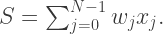
where the 


One technique which most data scientists proffer is to simulate many such Bernoulli draws and calculate quantiles empirically from the resulting simulations. This is possible, but the question is how much error is there in such simulations given arbitrary choices of
There is another approach: Using the Cornish-Fisher expansion, a technique dating from 1937. But before meeting the expansion, cumulants need to be introduced.
Cumulants
Technically, cumulants are the coefficients obtained from a series expansion of the log of the characteristic function of a probability density function. That’s dense. Let’s break it down.
The characteristic function is the expected value of a particular non-linear function of a random variable 


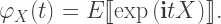
where 

If
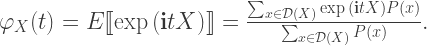
where 
Inspection shows these expressions are the value of a general Fourier transform of the probability density function, 
Taking the log, then

where (finally!) the 

roughly analogous to the moment generating function, or

where 


then

assuming cumulants exist for all 
This just sketches the beginning of things that can be done with cumulants. See k-statistics and polykays for others, even empirical uses.
The Cornish-Fisher expansion
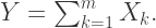
Given knowledge of cumulants, the Cornish-Fisher expansion gives an estimate for
Cumulants for 
The first five cumulants for each part, 
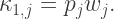
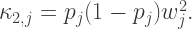
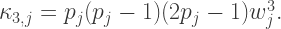


These are elemental cumulants and, so, to obtain the corresponding cumulants for
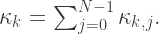
Note that
corresponds to the mean.
corresponds to the variance.
corresponds to skewness, hereinafter denoted
.
corresponds to kurtosis, hereinafter denoted
.
does not correspond to any central moment or simple combination of them.
Details are available here.
A Cornish-Fisher expansion for
library(mpoly)
theoreticalMean<- function(W,P) sum(W*P)
theoreticalVariance<- function(W,P) sum(W^2*P*(1-P))
theoreticalSkew<- function(W,P) sum(P*(P-1)*(2*P-1)*W^3)
# (This is not excess kurtosis. Still need to subtract 3 to get kurtosis w.r.t. Gaussian.)
theoreticalKurtosis<- function(W,P) sum(P*(1-P)*(1 + 6*P*(P - 1))*W^4)
theoreticalKappa5<- function(W,P) sum(P*(P-1)*(2*P-1)*(1 + 12*P*(1-P))*W^5)

gamma1<- function(W,P) theoreticalSkew(W,P)/sqrt(theoreticalVariance(W,P)^3)
gamma2<- function(W,P) theoreticalKurtosis(W,P)/sqrt(theoreticalVariance(W,P)^4)
gamma3<- function(W,P) theoreticalKappa5(W,P)/sqrt(theoreticalVariance(W,P)^5)

He.polynomials<- hermite(degree=1:4, kind="he", normalized=TRUE)
ThePoint<- 0.10
TheQuantile<- qnorm(ThePoint)

yAtThePoint<- function(xPoint=0.1, W, P)
{
  #
  xQuantile<- qnorm(xPoint)
  #
  He<- unlist(sapply(X=He.polynomials, FUN=function(He.k) as.function(He.k, silent=TRUE)(xQuantile)))
  #
  h1<- He[2]/6
  h2<- He[3]/24
  h11<- - (2*He[3]+He[1])/36
  h3<- He[4]/120
  h12<- -(He[4] + He[2])/24
  h111<- (12*He[4] + 19*He[2])/324
  #
  g1<- gamma1(W,P)
  g2<- gamma2(W,P)
  g3<- gamma3(W,P)
  #
  mu<- theoreticalMean(W,P)
  sigma<- sqrt(theoreticalVariance(W,P))
  #
  w<- xQuantile + (g1*h1) + (g2*h2 + g1^2*h11) + (g3*h3 + g1*g2*h12 + g1^3*h111)
  #
  yp<- mu + sigma*w
  #
  return(yp)
}
Simulating using many Bernoulli draws
A simulation for 


Comparing the two approaches


Comment on Cumulants and the Cornish-Fisher expansion in statistical education
Cumulants and the Cornish-Fisher expansion aren’t regularly taught any longer in courses on theoretical statistics, at least judging by material in statistics textbooks. For example,
- J. S. Bendat, A. G. Piersol, Random Data: Analysis and Measurement Procedures,
edition, Wiley, 2010
- A. W. Drake, Fundamentals of Applied Probability, McGraw-Hill Book Company, 1967
- J. A. Rice, Mathematical Statistics and Data Analysis,
edition, Duxbury, Thomson/Brooks/Cole, 2007
- M. H. DeGroot, M. J. Schervish, Probability and Statistics,
- K. V. Mardia, J. T. Kent, J. M. Bibby, Multivariate Analysis, Academic Press, 1979
- R. Durrett, Probability: Theory and Examples,
lack any mention of either cumulants or the expansion, although moment-generating functions are inevitably mentioned. In contrast,
- R. V. Hogg, J. W. McKean, A. T. Craig, Introduction to Mathematical Statistics,
edition, Pearson/Prentice-Hall, 2005
- A. N. Shiryaev, R. P. Boas (translator), Probability,
edition, Springer, 1996
- E. Parzen, Modern Probability Theory and Its Applications, John Wiley, 1960
- D. E. Knuth, The Art of Computer Programming, Volume 1: Fundamental Algorithms,
do mention cumulants. Parzen (1960) has quite a bit about them, and relationships to sums of random variables. The erudite Professor Knuth has three pages mentioning them. That suggests, however, that most specialists in computer science ought to know of them, but I’d bet most don’t.
Cumulants are often mentioned during courses on random walks and diffusion, because a random walk can be considered a kind of a sum.
Postscript
Should readers be interested in the code, I can prepare a documented version of it to use. Note that this would be in the interest of reproducibility. As mentioned above, the PDQutils package of R offers a means of calculating quantiles given cumulants directly, via its function qapx_cf. Of course, theoretical expressions for quantiles demand symbolic calculation, such as offered by the capabilities of Wolfram Mathematica.


