The title of this post is stolen from paper by Duncan Murdoch, Yu-Ling Tsai, and James Adcock which appeared in a 2008 issue of The American Statistician published by the American Statistical Association [August 2008, 62(3), 242-245]. Murdoch also has a presentation on the same subject where he recounts, among other experiences, a response from a medical journal when he objected to a mischaracterization of a p-value in one of their papers. Their paper is a riff off and extension of one by H. Sackrowitz and E. Samuel-Cahn, a 1999 paper in the same journal [called “p values as random variables — Expected p values”, 53(4), 326-331]. p-values are used in Neyman-Pearson hypothesis testing to decide between two competing hypotheses and, in fact, their hypothesis testing frame cannot be constructed unless there are two hypotheses, known and characterized in advance.

These papers make several points, the main being the stochastic nature of p-values as a statistical construct, notably that, the major point is that the distribution of the p-value conditional upon the Null Hypothesis being true is distributed over the unit interval. Conditional upon the alternative being true, a good test statistic is equivalent to a p-value which increases towards one. In consequence, Murdoch, Tsai, and Adcock point the silliness of certain interpretations of p-values when obtained. More about classical hypothesis testing can be found in a presentation by Slava Kharin “Statistical Concepts in Climate Research — Classical Hypothesis Testing”.

The older Fisherian view of p-values as a measure of an amount of inductive evidence against the Null Hypothesis is apparently still out there. (See the presentation by Kharin for more details about the Fisherian view. And see a Postscript just added to this post below expanding on this point.) The way p-values scatter over the unit interval under the true Null implies this interpretation is meaningless, certainly in point cases. I was therefore startled to re-encounter a blatantly wrong expression recently. Getting this is a really fundamental error in statistics, and should be enough to demand a revision of the statement by a referee.

In particular, as readers may know, I am working on studying “Overestimated global warming over the past 20 years”, a recent paper by Fyfe, Gillett, and Zwiers. In rough summary, this paper takes HadCRUT4 global temperature measurements and a set of CMIP5 climate model runs for the same period and points and tries to see how well the bunch of models did at predicting the observed temperature trends. I’ve been primarily trying to understand the procedure documented in their Supplement, or the methods used, and, since they relied upon bootstrap resampling techniques which I have spent some time studying, I wanted to see what they did. It’s a tough go, primarily because, from their Supplement, it is not clear how precisely they calculated trends. Nevertheless, I read the main body a couple of days ago and I was shocked to see:

Differences between observed and simulated 20-year trends have p values (Supplementary Information) that drop to close to zero by 1993–2012 under assumption (1) and to 0.04 under assumption (2) (Fig. 2c). Here we note that the smaller the p value is, the stronger the evidence against the null hypothesis. On this basis, the rarity of the 1993–2012 trend difference under assumption (1) is obvious. Under assumption (2), this implies that such an inconsistency is only expected to occur by chance once in 500 years, if 20-year periods are considered statistically independent. Similar results apply to trends for 1998–2012 (Fig. 2d). In conclusion, we reject the null hypothesis that the observed and model mean trends are equal at the 10% level.

The way they get one of the claims is to observed there are 25 20-year periods in 500 years and 1/.04 is 25. That’s not even the correct way of doing the calculation they want (see at bottom), but that’s beside the point. p-values are not chances of correctness of the Null or anything like that, nor can they be used to predict chances of extreme events. Perhaps the climate field is rife with this kind of abuse, but that does not justify it being here. (Murdoch found it is rife in medical literature, and, a personal communication I had recently with a physician researcher reports it remains true.)

Further, I have no idea where they get that “10% level” from. It is not in their main paper, appearing first in the quote above, and not in their cited Supplement. It is customary to set a level based upon a specific alternative, which apparently they do not have. I’m guessing they took the customary 5% and, because of the two-sided test, doubled it to get 10%, but I really do not know.

I am not (yet) quibbling with their results or methods, but this kind of presentation is just wrong and indicates a sloppy statistical review of the text. They got a near-zero p-value under assumption “(1)” and 0.04 under assumption “(2)”. That’s all they can say. They should say the estimate was done using bootstrap replications and how many were used, but that may be asking too much. The paper was, after all, a “Comment”, not a research report.

Postscript: 8th September 2013, 18:00 ET.

I was pretty dismissive of the Fisherian approach of “significant testing” above. Here’s why. This is an adaptation of the arguments presented by Westover, Westover, and Bianchi.

Suppose there’s an acquaintance who claims they can tell heads or tails accurately when flipping coin 10 times in a row. They seem upstanding, and they claim the coins are fair. You assess that the chance of their being a cheat or dishonest at a small probability d. You then observe this yourself, and, sure enough, they successfully predict the pattern the coin lands, some heads and some tails. Having a loaded coin seems unlikely. What’s the chance that they are dishonest?

Well, Fisherian significance testing says you approach this as follows. Disregard what you know or think of them. Calculate the chance of a fair coin landing in the predicted configuration, that chance being , and report that as the significance value. Your audience can decide whether or not that’s a likely outcome. (This is also discussed here, but I would recommend readers disregard the comments which are generally Way Off The Mark. See also a discussion of the base rate fallacy.) For every additional successfully predicted toss, the significance halves.

Now, if we use all the information we’re given, that the acquaintance is upstanding, and the coin is fair, we get a different result. Suppose we start by considering . To keep the formulas short, let the cheating case be abbreviated c, the not cheating case be abbreviated nc, and the observed “10 tossed guessed” as D for “Data”. Our Likelihood is just as in the case of the significance test, . And if there is cheating involved, . Then we can calculate:

.

Turning the crank,

.

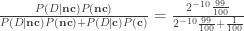
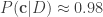
Well, that’s slightly less that 0.09. And, similarly,

.

That’s about 0.91.

Things are not looking so good for the acquaintance, but it’s not as severe as the significance test result. So, suppose we had a different ? How small would it need to be to match the significance test result? Suppose instead? Turning the crank again, and . Worse, as we’d expect. It ends up that if we end up with a result comparable to the significance test. This means, like it or not, the significance test is assuming a prior of , or, that the acquaintance has as much chance of being a cheat as not. There’s nothing said about that explicitly, but since it is equivalent to this case, and in fact can be derived from the Bayes’ Rule used, it’s entirely possible to interpret things this way. To do this is to ignore stuff we know, that is, not use all the information we have.

Postscript: 14th September 2013, 19:00 ET. Professor John Kruschke does a nice job showing the same kind of thinking in the Bayesian context, focussing upon choice among candidates and discussing how someone might pick a Likelihood (or Sampling Distribution) by examining data. Added 15th September 2013: Another example from Professor Kruschke.