This is a sketch of how maths and statistics can do something called blind source separation, meaning to estimate the components of data given only their totals. Here, I use Bayesian techniques for the purpose, sometimes called Bayesian inversion, using standard tools like the JAGS Gibbs sampler, and the programming language, R. I’ll present the problem and the solution, and then talk about why it works.

Getting residents of a town to reduce their solid waste production can be an important money saver for towns, many of which are paying $80 per ton or more for solid waste disposal and hauling. Much effort is spent convincing them to recycle materials that are eligible, and to do other things, like household composting which reduces weight a lot due primarily to the latent water in household garbage scraps.

But outreach programs only work if residents can be successfully contacted, and this can be difficult in suburban settings. Moreover, blanket advertising and promotions can themselves be costly and may be ineffective. As in other marketing, it is better to identify target populations and focus messaging on them. In this case, for a town, identifying households which produce more per unit tonnage is attractive, and outreach can be limited to them. Unfortunately, tonnage by household is not generally available to towns. Even tonnage by street is typically not reported by haulers. What is reported is total tonnage by route, or something comparable.

While this sketch is simplified for ease of understanding, and an actual analysis of trash routes would require more effort and details, it shows how such separation can be done. I also don’t have actual control tonnage for a set of houses. (I do have route tallies.) Thus, the technique used for illustration is simulation of synthetic data where the contribution of individual houses is known by design. The objective is to see if the Bayesian inversion can recover the components.

For the purpose I posit that there are two streets in a neighborhood, one have 5 homes, the other having 7 homes. The hauler reports weekly solid waste tonnage for the combination of both streets. There is a year’s worth of data. Generally speaking, larger homes produce more waste, where “larger” can mean more people or bigger houses or higher income per home member. Also, generally speaking, the variability in tonnage each week is higher the more trash is produced. The same kind of model can be applied to recycling tonnage, but here I’m limiting the study to trash. In particular, image that the two streets are arranged as in the following figure. The numbers indicate the amount of solid waste produced by the nearby home per week. The units are in tens of kilograms.

(Click on figure to see larger image.)
Mean values per week for the hours were chosen by modeling each street with a Poisson, and picking a different mean for each. Specifically,

SevenHomeMeans<- rpois(n=7, lambda=1.6*10)/10
FiveHomeMeans<- rpois(n=5, lambda=2.3*10)/10


I model variability by positing that the coefficient of variation for each home is constant, so the standard deviation in variability is proportional to their mean. In particular, I’ve picked a somewhat arbitrary 1.2 for the coefficient of variation, intending to capture the variation across major holidays. The model assumes no correlation week to week per home, either in the simulation or in the recovery. There is a town wide correlation easily seen across the November-December holidays, but how strong this is at a household level is not at all clear. The technique should work nevertheless, but these synthetic data do not demonstrate that.

52 observations are drawn for each of the houses, via

SevenHomeMeans<- c(1.7, 1.7, 1.4, 1.0, 2.7, 1.8, 1.5)
FiveHomeMeans<- c(2.2, 3.4, 2.7, 2.5, 1.6)

ySevenHomes<- t(sapply(X=1:7, FUN=function(k) abs(rnorm(n=N, mean=SevenHomeMeans[k], sd=sdSevenHomes[k]))))
yFiveHomes<- t(sapply(X=1:5, FUN=function(k) abs(rnorm(n=N, mean=FiveHomeMeans[k], sd=sdFiveHomes[k]))))


Then the results are added to get each street’s tonnage for the year, and the tonnage for the streets added to get the composite, confounded tonnage, in y.

y7<- colSums(ySevenHomes)
y5<- colSums(yFiveHomes)
y<- y5+y7

The resulting dataset looks like:

(Click on figure to see larger image.)
If the data contributing to these totals from the individual streets are displayed on the same scatterplot, it looks like:

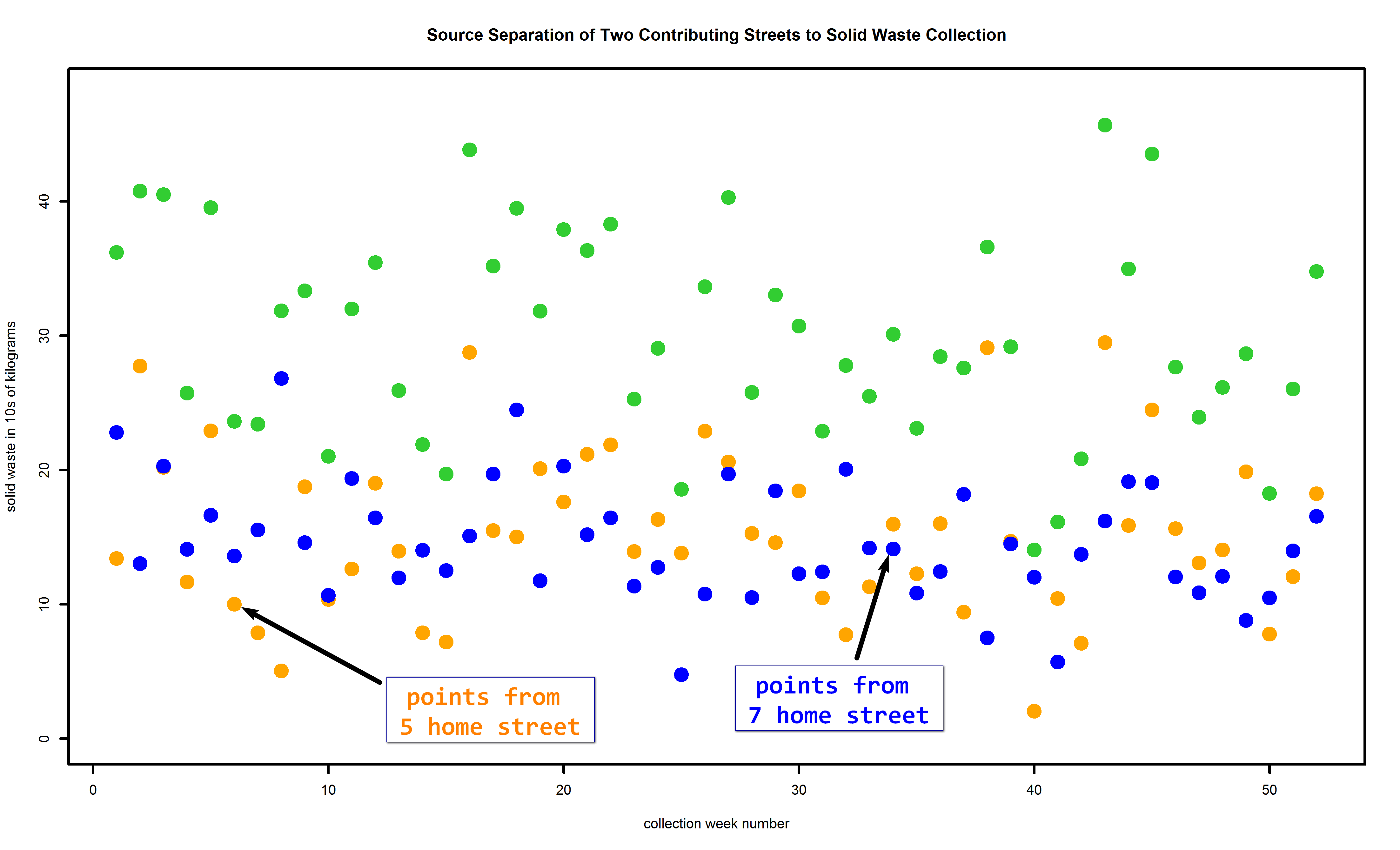
(Click on figure to see larger image.)
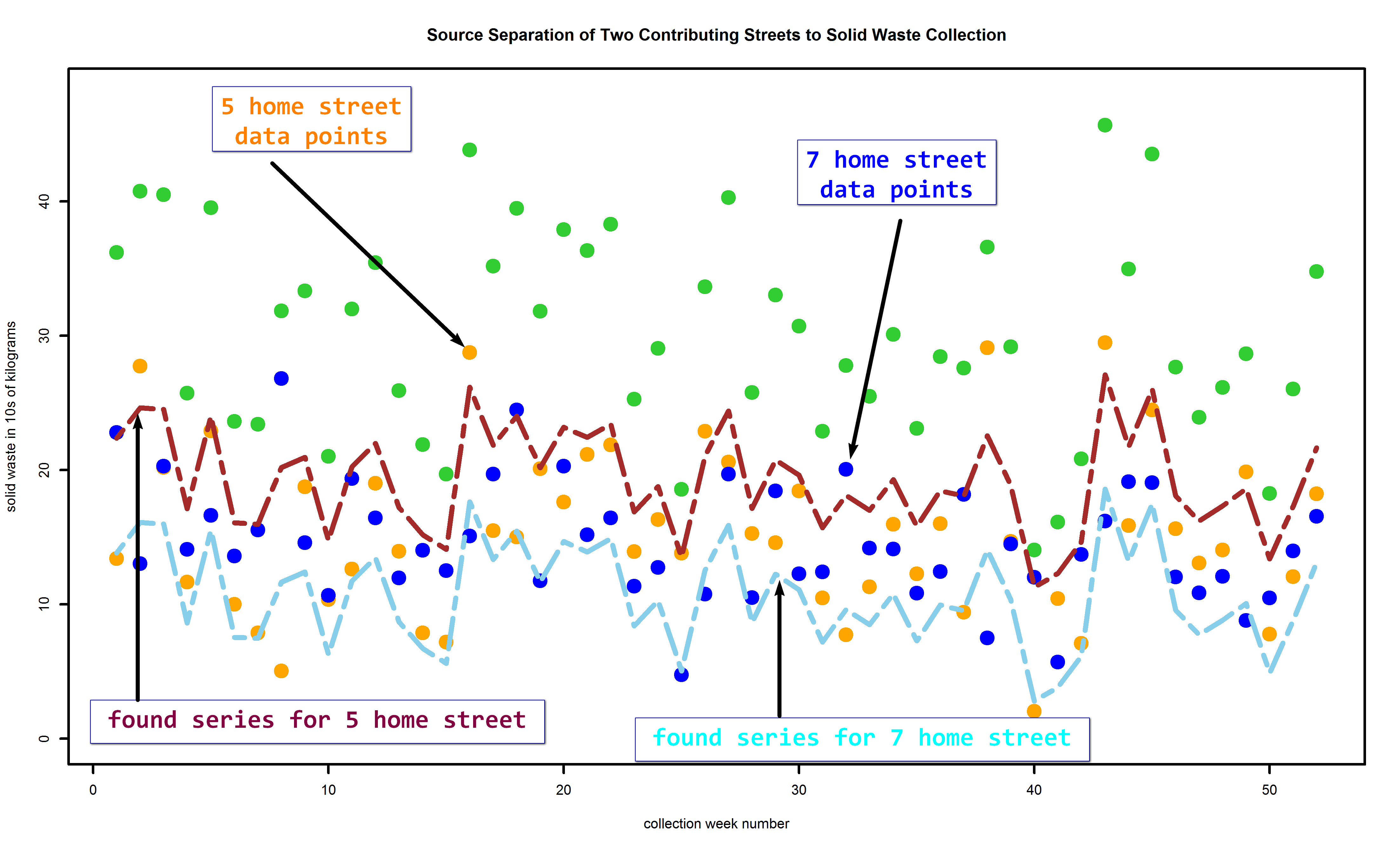
Of course, the Bayesian inversion does not know these … It’s trying to figure these out. And, in fact, it does that pretty well:

(Click on figure to see larger image.)
The maroon trace is the algorithm’s estimate of the higher street in terms of tonnage, the 5 home street. The aqua or skyblue trace is the estimate of the lower street’s tonnage. While these do not go through all the corresponding dots, especially in their extremes, the estimates follow the trends pretty well. The estimates also are sometimes early when there’s an uptick or downtick, and sometimes late, about one or two weeks at most.

The point is to find out which street should receive more educational materials and tutoring regarding solid waste reduction. Detailed predictions by week aren’t really needed for that. All that’s really needed are estimates of the overall means for each street separately. The algorithm finds that, but the week by week breakouts are a bonus.

(Click on figure to see larger image.)
Here the pinkish red dashed line corresponds to the estimate of the mean of the higher tonnage street, and the navy blue dashed line to the estimate of the mean of the lower tonnage street.

Lastly, it’s good to see that the sum of the estimates of the individual streets for each week match the data very closely.

(Click on figure to see larger image.)
Now, a bit of fun. We can watch the Gibbs sampler in action. First, upon startup, the sampler is initialized and that initialization is (typically) far from any solution. The movie shows how the algorithm explores and eventually finds the area of plausible solutions for breaking tonnage into components.

Once that region is found, the algorithm spends a lot of time trying various combinations that add up to the totals of the data, in order to estimate the best overall mix.

The code and data for these calculations are available in a gzip’d tarball. It includes the code for making the movies, but these require software not included, such as ImageMagick tools. Also, the code is not portable, offered as is from the version generating this example on my 64-bit Windows 7 system.

The technical details of the Bayesian hierarchical model are given below.

The value of the combined tonnage at each point is the sum of two components, both modeled as Gaussians having distinct means and standard deviations. Both standard deviations have a common hyperprior as their model, a Gamma distribution with shape 3 and rate 0.005. The means, however, are products of a , a random variable specific to component , and another random, called in the code, which represents how much total tonnage is produced at the time point. is modeled as a uniform random variable having a value between 10 and 500 kilograms. The random variables, are taken from a partial stick-breaking process. That means is drawn from a uniform on the unit interval, and is drawn on the interval zero to . The remainder of the unit interval is ignored. This mechanism keeps and separated and, thereby, the means of the two components, identified in the code as and . Finally,
the total at each time point is the sum of the components and the zero-crossings trick is used to constrain it close to the data , by saying

data
{
for (i in 1:N)
{
z[i]<- 0
}
}
model
{
.
.
.
for (i in 1:N)
{
for (j in 1:M)
{
yc[i,j] ~ dnorm(mu[j], tau[j])
}
tally[i]<- sum(yc[i,1:M])
z[i] ~ dnorm(y[i] - tally[i], 30)
}
.
.
.
}


So, why does this work?

The statistics of the waste production of the homes on the 5 house street are markedly different than those of the 7 house street. Because of that, there is a clear way to cluster and separate the two streets. Were the statistics more to overlap — and this would mean in both means and in variability — this separate would be more difficult. Note that if the means were the same but the standard deviations of waste tonnage markedly different between the two streets but consistent on the same street, that would suffice to separate.

There are ways of doing the separation using frequentist methods, notably using the SVMs of machine learning, but I think Bayesian separation is more straightforward and cleaner.